In Code We Trust: Why your computer makes mistakes
Fast and Spurious
It is well-known that our computers can perform operations at a dizzying speed. The miniaturization of transistors has continuously and dramatically increased their performance. The computer I am using to write these lines can perform several hundred million arithmetic operations per second. Parallelism is another source of improvement for computing speed. The available software libraries in various programming languages today integrate all the necessary tools to develop parallel code on CPU and/or GPU.
With these observations in mind, a question arises: are the computations performed by our computers accurate? The answer to this question is very clear: computers can "make mistakes". In fact, not only do they make mistakes, but they make mistakes very often, if not always. Perhaps this statement is a little unfair and inaccurate, after all, they are meticulously following a set of rules for which they were designed. In this blog article, I will give a brief overview of these rules while discussing the source of numerical errors. We will also address some effective strategies developed to overcome them. But to start with, let’s dive into the representation of numbers used within our computers.
Close Counters of the Third Kind
The decimal system dates to ancient times, but it is not the one favored by our computers, which, as another well-known fact, only manipulate 0s and 1s, called “bits.” To go a little further, we need to do some elementary mathematics. One can show indeed that any real number x can be theoretically written in the form:
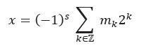
where s, mk ∈ {0,1}. This decomposition is called binary representation and is used by most of our computers. Two important things are to be noted: first, the number of terms appearing in the sum may be finite or not. The second is that every real number can be fully described by the value of its sign bit s and the sequence {mk}k ∈Z consisting of 0s and 1s. It is obvious that a computer, no matter how powerful, cannot store an infinite number of 0's and 1's, thus limiting the set of representable real numbers. The set of numbers manipulated by our computers are called floating-point numbers. If you are not familiar with them, allow me to introduce you.
To make things easier, let's take an example, let's say x = 5.75. Its decomposition in base 2 is written as follows:
5.75 = 22 + 20 + 2-1 + 2-2 = (101.11)base 2
Let's factor out the largest "component" in the decomposition, which is 22 in this case:
5.75 = 22 ⋅ (1 + 2-2 + 2-3 + 2-4 ) = (22 ⋅ 1.0111)base 2
In this format, called normalized representation, we see the following more general form appear:
x = (-1)s ⋅ 2N ∙ (1 + m-1 2-1 + ⋅⋅⋅ + m-n 2-n)
This representation suggests that by storing the sign bit s, the integer N called exponent, and the sequence of bits {m-1, ⋅⋅⋅, m-n} called mantissa, we can unambiguously represent the number x. Note that integer N must also be decomposed in base 2, which ultimately amounts to saving a second sequence of bits, precisely what our computers do.
The Rules of The Game
The field of floating-point arithmetic is not only concerned with the representation of numbers. As we want to perform calculations, it has been necessary to develop effective and implementable methods on processors to achieve this purpose. Until the 1980s, each processor manufacturer had its own implementation which was not without its problems. For instance, even elementary calculations could vary from one system to another, resulting (among other problems) in reproducibility issues. It was not until 1985 that a standard finally appeared, namely the IEEE 754 standard, largely thanks to the work of Professor William Kahan, "The Father of Floating Point". This standard defines the formats for different types of numbers, the behavior and precision of basic operations (+,-,*,/,√), as well as elementary functions, special values, rounding modes and exception management. In 2008 it underwent a significant revision and again in 2019. It is very likely that the computer you are using implements this standard like most current computers.
Mad Math
In the following, I will try to give you an idea of the amount of double-precision floating-point numbers a 64-bit computer can handle. Let's start by schematically visualizing the distribution of a subset of the representable floating-point numbers (we only represent the positive part as the situation is symmetric on the negative one):
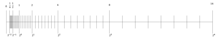
The first observation we can make is that the number of floating-point numbers is the same on each interval of the form [2k,2(k+1) ┤[ for k belonging to Z.
In other words, the density of floating-point numbers decreases towards large numbers.
In double precision on a 64-bit system, do you have an idea of how many are in the interval [1,2[ ? There are 252 of them which is 4 503 599 627 370 496, —much more than the 100 billion stars in our galaxy! The difference between two consecutive floating-point numbers in this range is 2(-52)≈2.22 10(-16) (as a reminder, the size of a proton in meters is approximately 1.68 10(-15) meters). Let's continue our dive: if we push our computer to its limits, the smallest positive floating-point number (in denormalized mode) is on the order of 4.94 10(-324).
On the other end of the spectrum, when we reach the last representable numbers, the distance between two consecutive floating-point numbers is of the order of 1.99584 10292 (according to the latest news, the radius of the observable universe was of the order of 8.8 1026) until reaching the maximum value of approximately 1.79769 10308.
True Lies
As we mentioned, our computers "make errors" in calculations. The graph illustrating the distribution of floating-point numbers is very helpful in understanding the reasons for this. Let's consider an example. We take two floating-point numbers x and y and perform any arithmetic operation. Let x⊙ y denote the theoretical result of this operation. What do we observe?
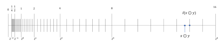
We observe that the machine cannot represent the theoretical result.
The best we can hope for is that the returned result is as close as possible to the correct result. This desirable property called the correct rounding yields the result noted "◊" (x⊙y) in the chart. Although this property is guaranteed by the IEEE standard for basic arithmetic operations (and square root), it remains that we obtain an approximate result.
Let's consider another example illustrating the absorption phenomenon. We are asking our computer to calculate the sum of the two floating-point numbers x and dx represented in the graph below:
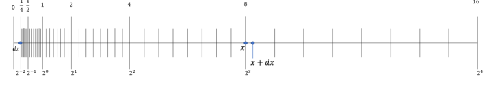
As the theoretical value cannot be represented by a floating-point number, the exact rounding rule applies leading to "◊" (x+dx)=x. Not really what we would have expected…
In the field of computational geometry, which is my area of work, numerical errors can have very sensitive negative effects. Let me illustrate this with the concept of predicate. In simple terms, a predicate is a computer program that returns true or false. Most algorithms performing geometric calculations rely on a series of predicates that act as switchers: based on their responses, the program will follow a path, perform calculations until the next predicate is reached. Suppose now that due to numerical errors, one of the predicates returns the wrong answer. The switch redirects us onto the wrong track… If the program ends, the result may not meet our expectations, but the consequences can be far worse: imagine for instance a program performing tests whose results are mutually contradictory. It might run towards dark destinies…
Some Like It Exact!
I used to believe that numerical errors were a curse that one had to learn to live with. Most of the geometry code I had been exposed to until then dealt with the sneaky consequences of rounding errors in their own way, developing often very clever strategies. It was while studying mesh generation algorithms that I discovered what I had believed until then was impossible: a computer can calculate exactly. There is indeed a branch of mathematics that develops sophisticated methods to achieve this. In the following, I will give a flavor of two of those methods.
The first one consists of dynamically expanding the memory space required to represent new floating-point numbers. Since a floating-point number is built upon two integers (mantissa, exponent, the sign being a bit), the method begins by extending the representation of integers in arbitrary precision. If an integer takes up 32 bits on our machine, any integer x can be represented by an array a[0], …, a[n] (of integers) such that:
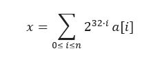
Then, this new set of integers of arbitrary length must be equipped with basic algebraic operations, which can be easily performed. Endowed with this, the arithmetic operations (+, -, *, /) can finally be implemented on the extended floating-point numbers.
The second technique I wanted to mention is also based on a particular decomposition called expansion. Here a real number x is decomposed in the form:
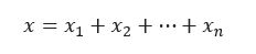
where x1>⋯>xn are regular floating-point numbers and satisfying a technical property called the non-overlapping property. Just as the previous method with the extended floating-point numbers, advanced algorithms have been designed to compute and perform arithmetic operations with expansions. Now comes the crucial point:
the non-overlapping property ensures that the signs of x (the theoretical result) and x1 (the largest term of the expansion which is actually computed) are the same. As a predicate can be formulated as a simple sign test on x, it is safe to use x1 instead! Implemented with expansions, the predicates will “mathematigically” never lie to us.
Naturally, despite all the efforts and ingenuity put into developing these techniques, they have their own limits. In particular, they remain constrained by the available memory on the computer. Furthermore, computation times using these techniques remain significantly longer than in fixed precision arithmetic, which implies a careful usage.
The BFGs
I read somewhere that mathematician Alston Householder may have said or written, “It makes me nervous to fly on airplanes since I know they are designed using floating point arithmetic.” I don't know if Professor Householder had reassured himself with the emergence of the IEEE standard and the sophistication of the numerical methods to which he contributed so much. What is certain, however, is that thanks to the work of giants such as Herbert Edelsbrunner, Douglas Priest, Jean-Daniel Boissonnat, Jonathan Shewchuk, Bruno Levy, and many others, scientific developers now have access to software libraries that allow them to deal with the effects of numerical errors more safely. The software solutions on which I work on daily have greatly benefited from the techniques discussed in this blog post, increasing their robustness and reliability. Is it the end of the story though? Certainly not, as other tracks have been proposed and the creativity of researchers and engineers in this field is seemingly inexhaustible.
Sources
- Edelsbrunner, Herbert, and Ernst Peter Mücke. "Simulation of simplicity: a technique to cope with degenerate cases in geometric algorithms." ACM Transactions on Graphics (tog) 9.1 (1990): 66-104.
- Fortune, Steven, and Christopher J. Van Wyk. "Efficient exact arithmetic for computational geometry." Proceedings of the ninth annual symposium on Computational geometry. 1993.
- Gustafson, John L. The end of error: Unum computing. CRC Press, 2017.
- Lafage, Vincent. "Revisiting" What Every Computer Scientist Should Know About Floating-point Arithmetic"." arXiv preprint arXiv:2012.02492 (2020).
- Lévy, Bruno. "Robustness and efficiency of geometric programs: The Predicate Construction Kit (PCK)." Computer-Aided Design 72 (2016): 3-12.
- Richard Shewchuk, Jonathan. "Adaptive precision floating-point arithmetic and fast robust geometric predicates." Discrete & Computational Geometry 18 (1997): 305-363.
Author Information:
Emmanuel Malvesin started his career at Ansys (Villeurbanne, France) as a scientific computing engineer, working in the computational geometry domain (mesh morphing, surface reconstruction). In 2011, he joined the SLB Montpellier Technology Center in the Structural Modeling team, where he discovered the field of geosciences. At the confluence of mathematics, physics, and computer science, his activities take him from the meshless world to the boundary elements, and ultimately to the depths of the machine.

Emmanuel Malvesin
Geoscientist
SLB Montpellier Technology Center
Related products
Harness the power of liberated data, AI, and leading software applications on the cloud based Delfi digital platform. Drive innovation with solutions across exploration, development, drilling, production, and new energy operations.
We work with your teams to accelerate progress to fully deployed enterprise-scale digital solutions, maximizing the potential of data, AI, and digital solutions for your business.